Originally posted on the Google AI Blog.
Many of the world's toughest scientific challenges, like developing
high-temperature superconductors and understanding the
true nature of space and time, involve dealing with the complexity of quantum systems. What makes these challenges difficult is that the number of
quantum states in these systems is exponentially large, making brute-force computation infeasible. To deal with this, data structures called
tensor networks are used. Tensor networks let one focus on the quantum states that are most relevant for real-world problems—the states of low energy, say—while ignoring other states that aren't relevant. Tensor networks are also increasingly finding applications in machine learning (ML). However, there remain difficulties that prohibit them from widespread use in the ML community: 1) a production-level tensor network library for
accelerated hardware has not been available to run tensor network algorithms at scale, and 2) most of the tensor network literature is geared toward physics applications and creates the false impression that expertise in quantum mechanics is required to understand the algorithms.
In order to address these issues, we are releasing
TensorNetwork, a brand new open source library to improve the efficiency of tensor calculations, developed in collaboration with the
Perimeter Institute for Theoretical Physics and
X. TensorNetwork uses
TensorFlow as a backend and is optimized for
GPU processing, which can enable speedups of up to 100x when compared to work on a CPU. We introduce TensorNetwork in a series of papers, the
first of which presents the new library and its
API, and provides an overview of tensor networks for a non-physics audience. In our
second paper we focus on a particular use case in physics, demonstrating the speedup that one gets using GPUs.
How are Tensor Networks Useful?
Tensors are multidimensional arrays, categorized in a hierarchy according to their
order: e.g., an ordinary number is a tensor of order zero (also known as a
scalar), a
vector is an order-one tensor, a
matrix is an order-two tensor
Diagrammatic notation for tensors. and so on. While low-order tensors can easily be represented by an explicit array of numbers or with a mathematical symbol such as T
ijnklm (where the number of indices represents the order of the tensor), that notation becomes very cumbersome once we start talking about high-order tensors. At that point it's useful to start using diagrammatic notation, where one simply draws a circle (or some other shape) with a number of lines, or legs, coming out of it—the number of legs being the same as the
order of the tensor. In this notation, a scalar is just a circle, a vector has a single leg, a matrix has two legs, etc. Each leg of the tensor also has a
dimension, which is the size of that leg. For example, a vector representing an object's velocity through space would be a three-dimensional, order-one tensor.
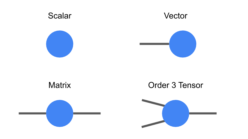 |
| Diagrammatic notation for tensors. |
The benefit of representing tensors in this way is to succinctly encode mathematical operations, e.g., multiplying a matrix by a vector to produce another vector, or multiplying two vectors to make a scalar. These are all examples of a more general concept called
tensor contraction.
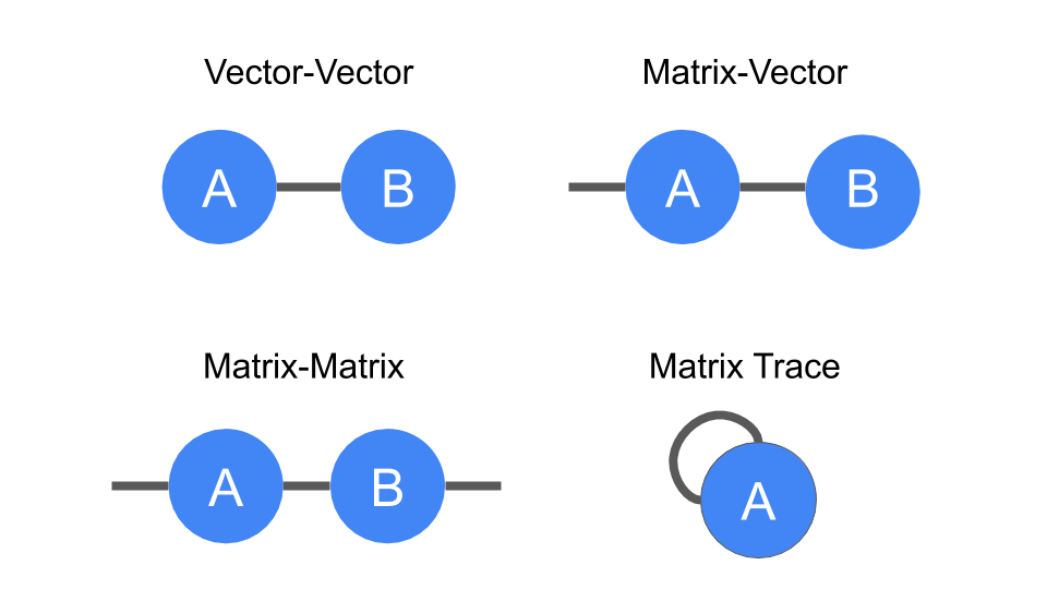 |
| Diagrammatic notation for tensor contraction. Vector and matrix multiplication, as well as the matrix trace (i.e., the sum of the diagonal elements of a matrix), are all examples. |
These are also simple examples of
tensor networks, which are graphical ways of encoding the pattern of tensor contractions of several constituent tensors to form a new one. Each constituent tensor has an order determined by its own number of legs. Legs that are connected, forming an edge in the diagram, represent contraction, while the number of remaining dangling legs determines the order of the resultant tensor.
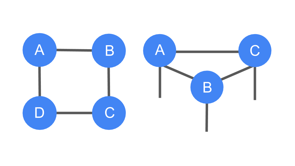 |
| Left: The trace of the product of four matrices, tr(ABCD), which is a scalar. You can see that it has no dangling legs. Right: Three order-three tensors being contracted with three legs dangling, resulting in a new order-three tensor. |
While these examples are very simple, the tensor networks of interest often represent hundreds of tensors contracted in a variety of ways. Describing such a thing would be very obscure using traditional notation, which is why the
diagrammatic notation was invented by Roger Penrose in 1971.
Tensor Networks in Practice
Consider a collection of black-and-white images, each of which can be thought of as a list of
N pixel values. A single pixel of a single image can be
one-hot-encoded into a two-dimensional vector, and by combining these pixel encodings together we can make a 2^
N-dimensional one-hot encoding of the entire image. We can reshape that high-dimensional vector into an order-
N tensor, and then add up all of the tensors in our collection of images to get a total tensor
Ti1,i2,...,iN encapsulating the collection.
This sounds like a very wasteful thing to do: encoding images with about 50 pixels in this way would already take
petabytes of memory. That's where tensor networks come in. Rather than storing or manipulating the tensor
T directly, we instead represent
T as the contraction of many smaller constituent tensors in the shape of a tensor network. That turns out to be much more efficient. For instance, the popular
matrix product state (MPS) network would write
T in terms of
N much smaller tensors, so that the total number of parameters is only linear in
N, rather than exponential.
 |
| The high-order tensor T is represented in terms of many low-order tensors in a matrix product state tensor network. |
It's not obvious that large tensor networks can be efficiently created or manipulated while consistently avoiding the need for a huge amount of memory. But it turns out that this is possible in many cases, which is why tensor networks have been used extensively in quantum physics and, now, in machine learning.
Stoudenmire and Schwab used the encoding just described to make an image classification model, demonstrating a new use for tensor networks. The TensorNetwork library is designed to facilitate exactly that kind of work, and our
first paper describes how the library functions for general tensor network manipulations.
Performance in Physics Use-Cases
TensorNetwork is a general-purpose library for tensor network algorithms, and so it should prove useful for physicists as well. Approximating quantum states is a typical use-case for tensor networks in physics, and is well-suited to illustrate the capabilities of the TensorNetwork library. In our
second paper, we describe a
tree tensor network (TTN) algorithm for approximating the ground state of either a periodic quantum spin chain (1D) or a lattice model on a thin torus (2D), and implement the algorithm using TensorNetwork. We compare the use of CPUs with GPUs and observe significant computational speed-ups, up to a factor of 100, when using a GPU and the TensorNetwork library.
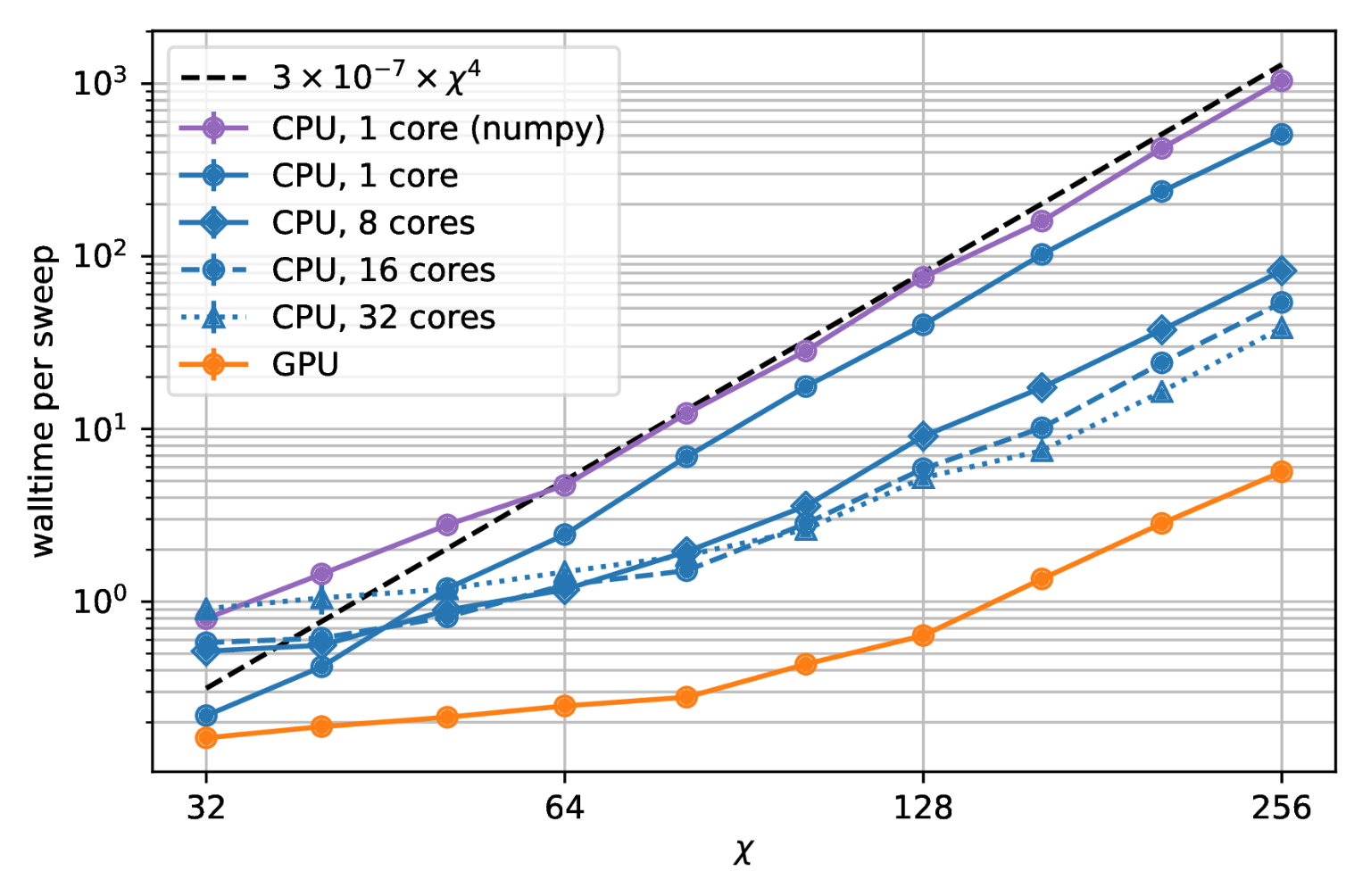 |
| Computational time as a function of the bond dimension, χ. The bond dimension determines the size of the constituent tensors of the tensor network. A larger bond dimension means the tensor network is more powerful, but requires more computational resources to manipulate. |
Conclusion and Future Work
These are the first in a series of planned papers to illustrate the power of TensorNetwork
in real-world applications. In our next paper we will use TensorNetwork to classify images in the
MNIST and
Fashion-MNIST datasets. Future plans include time series analysis on the ML side, and quantum circuit simulation on the physics side. With the open source community, we are also always adding new features to TensorNetwork itself. We hope that TensorNetwork will become a valuable tool for physicists and machine learning practitioners.
Acknowledgements
The TensorNetwork library was developed by Chase Roberts, Adam Zalcman, and Bruce Fontaine of Google AI; Ashley Milsted, Martin Ganahl, and Guifre Vidal of the Perimeter Institute; and Jack Hidary and Stefan Leichenauer of X. We'd also like to thank Stavros Efthymiou at X for valuable contributions.
by Chase Roberts, Research Engineer, Google AI and Stefan Leichenauer, Research Scientist, X